4. B-Trees

B-trees are an immensely powerful tools that are used in SQL and in filesystems. They inherited a loft from red-black trees. Let us figure out what they are and how they work.

B-trees are balanced search trees designed to work well on disks or other direct-access secondary storage devices. B-trees are like red-black trees, but they are better at minimizing disk I/O operations. Many database systems use B-trees, or variants of B-trees, to store information.

B-trees differ from red-black trees in that B-tree nodes may have many children, from a few to thousands. That is, the "branching factor" of a B-tree can be quite large, although it usually depends on characteristics of the disk unit used. B-trees are similar to red-black trees in that every n-node B-tree has height O(lgn) The exact height of a B-tree can be less than that of a red-black tree, however, because its branching factor, and hence the base of the logarithm that expresses its height, can be much larger. Therefore, we can also use B-trees to implement many dynamic-set operations in time O(lgn).

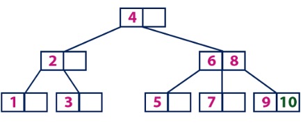
B-trees generalize binary search trees in a natural manner. Next image shows a simple B-tree. If an internal B-tree node x contains x[n] keys, then x has x[n] + 1 children. The keys in node x serve as dividing points separating the range of keys handled by x into x[n] C 1 subranges, each handled by one child of x. When searching for a key in a B-tree, we make an (x[n] + 1)-way decision based on comparisons with the x[n] keys stored at node x. The structure of leaf nodes differs from that of internal nodes; we will examine these differences.

Figure 5.1

A B-tree T is a rooted tree (whose root is T.root) having the following properties:

• Every node x has the following attributes:
  • x[n], the number of keys currently stored in node x
  • the x.n keys themselves, x[key[1]]; x[key[2]], …, x[key[x[n]]], stored in nondecreasing order, so that x[key[1]] ≤ x[key[2]] ≤ … ≤ x[key[x[n]]]
  • x.leaf, a boolean value that is true if x is a leaf and false if x is an internal node.
• Each internal node x also contains x[n] + 1 pointers x[c[1]];x[c[2]]; … ;x[c[x[n] + 1]] to its children. Leaf nodes have no children, and so their c[i] attributes are undefined.
• The keys x[key[i]] separate the ranges of keys stored in each subtree: if k[i] is any key stored in the subtree with root x[c[i]], then: k1 ≤ x[key[1]] ≤ k[2] ≤ x[key[2]] ≤ … ≤ x[key[x[n]]] ≤ k[x[n] + 1]
• All leaves have the same depth, which is the tree's height h
• Nodes have lower and upper bounds on the number of keys they can contain. We express these bounds in terms of a fixed integer t ≥ 2 called the minimum degree of the B-tree:
  • Every node other than the root must have at least t - 1 keys. Every internal node other than the root thus has at least t children. If the tree is nonempty, the root must have at least one key.
  • Every node may contain at most 2t - 1 keys. Therefore, an internal node may have at most 2t children. We say that a node is full if it contains exactly 2t - 1 keys.

To perform an insertion follow this procedure:

• Check if the tree is empty.
• If tree is empty, create a new node with inserted value and use it as root of the tree.
• If tree is not empty, find an appropriate leaf node to append the value by using b-tree search algorithm.
• If found element has an empty position, add new value to the node, following nondecreasing order.
• If found element is full, split the leaf node, while sending the middle value to the parent. Repeat this process until sent value is added to a node.
• If split is performed on a root node, then create a new root node and add the middle value into it. The tree height is then increased by 1.

Following is an example of adding values 1 through 10 to a b-tree.

Add element 1 by creating a root node.

Figure 5.2

Add element 2 by adding it to a root node.

Figure 5.3

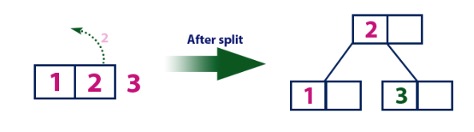
Add element 3 by splitting root node.

Figure 5.4

Add element 4 by adding it to the appropriate leaf.

Figure 5.5

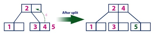
Add element 5 by splitting node with 3 and 4.

Figure 5.6

Add element 6 to the appropriate leaf.

Figure 5.7

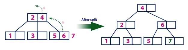
Add element 7 to appropriate leaf. Then split the leaf and send middle value (6) up.

Figure 5.8

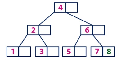
Add element 8 to appropriate leaf.

Figure 5.9

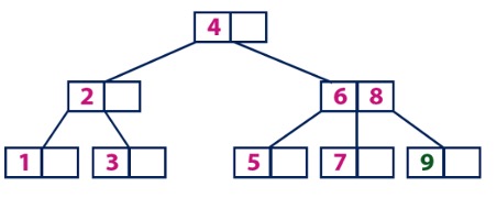
Add element 9 to leaf with values 7 and 8. Split the node and send the 8 upwards.

Figure 5.10

Add value 10 to node with 9.

Figure 5.11